Pairs trading with financial spread betting involves buying one market and selling another to trade their relative performance. A trader might buy a share judged temporarily weak compared with a related share, while selling the stronger one in the expectation that the relationship will recover. Profit depends on how the two positions perform together after costs, rather than simply whether the wider market rises or falls. The approach can reduce some shared market exposure, but it introduces risks involving the relationship, sizing and execution of both trades. This guide explains how pairs trading works, who it may suit, how to calculate stakes and how to assess realistic winning and losing outcomes.
A long position and a short position do not automatically create a safe or market-neutral arrangement. Both can lose at the same time, and each can require margin and incur holding costs. The Financial Conduct Authority includes spread betting within its CFD product supervision and describes these leveraged products as high risk and unsuitable for some retail consumers. The examples in this article use hypothetical prices, relationships and charges for education. They do not identify recommended trades or promise that a historical relationship will return. Before placing a real pair, understand both contracts separately and calculate the combined exposure, costs and potential losses under several different market conditions.
What Is Pairs Trading?
A pairs trade contains two positions, often called legs: a long position in one instrument and a short position in another. The central idea is that one will perform better than the other over the holding period, after allowing for their relative sizes. In a common mean-reversion approach, the trader buys the instrument considered relatively cheap and sells the one considered relatively expensive. Those descriptions refer to a defined relationship, not necessarily to fundamental investment value. A lower share price alone does not make a company cheaper. Different share counts, capital structures and business prospects make a simple comparison of two companies’ quoted prices an inadequate basis for a trade.
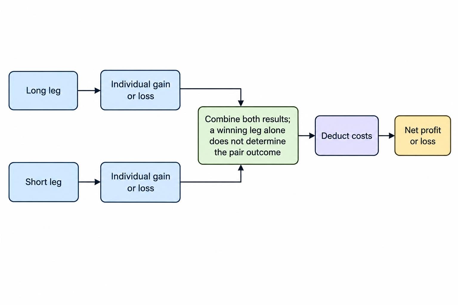
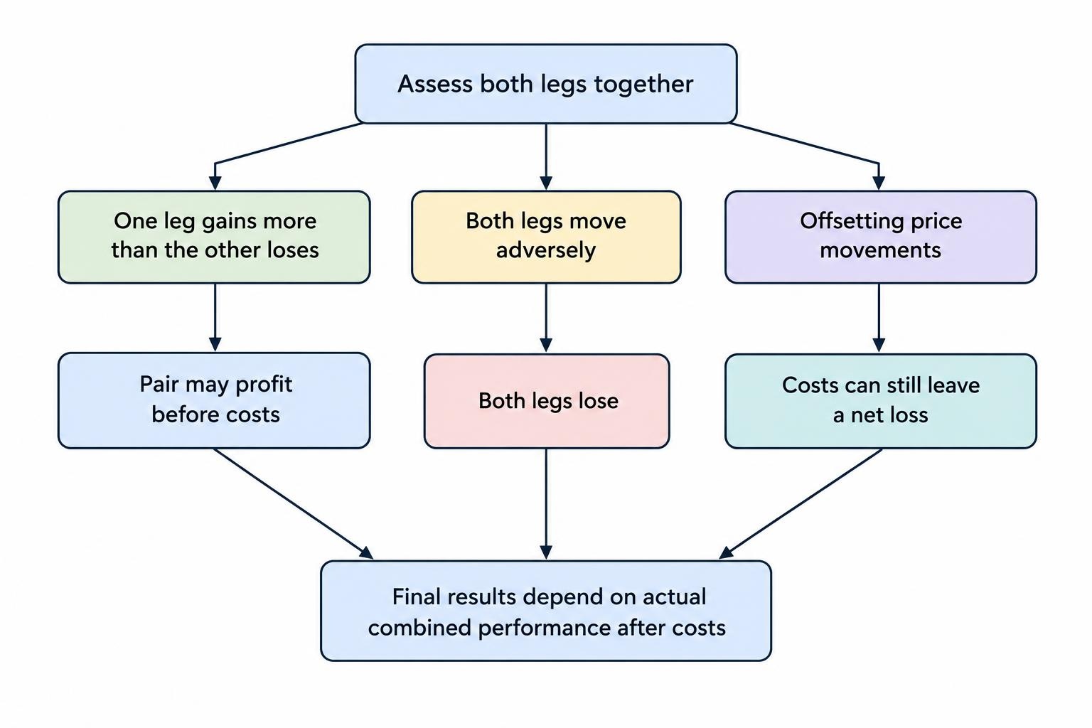
The outcome must be calculated across both legs. If the long gains £100 and the short loses £40, the pair has made £60 before costs. If the long loses £30 while the short gains £80, the pair has made £50 before costs even though both underlying markets may have fallen. Conversely, a £100 gain on one leg cannot rescue a £150 loss on the other. This combined view is central to the strategy and should continue through entry, monitoring and exit. Treating the profitable leg as a success while ignoring the other position gives a misleading account of performance and can encourage poor decisions about when to close the pair.
Pairs Trading, Hedging and Relative Momentum
Pairs trading often uses some of the same mechanics as hedging, but the objective can differ. A hedge usually aims to reduce a particular risk in an investment or exposure already held. A pairs trader commonly opens both positions to seek a return from their relative movement. Calling the short leg a hedge does not establish that it offsets every risk in the long leg. Both instruments can remain exposed to company announcements, changing sector conditions or different economic drivers. The trader must specify whether the goal is to reduce broad market sensitivity, capture a relative valuation change or pursue a statistically defined relationship, because those objectives lead to different sizing and exit choices.
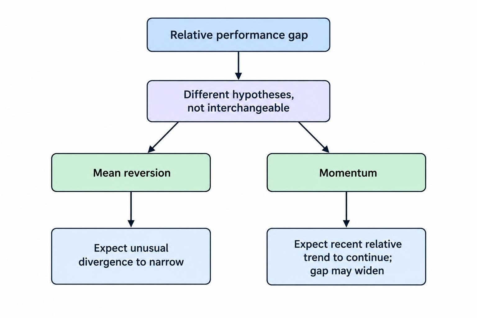
Mean reversion is not the only way to construct a relative trade. A momentum approach can buy the recent relative winner and sell the relative loser, expecting their performance gap to continue widening. A mean-reversion pair normally takes the opposite view, expecting an unusual divergence to narrow. These are different hypotheses, and switching between them after a loss changes the strategy. A widening relationship cannot be treated as evidence to hold indefinitely under whichever explanation feels convenient. This guide concentrates on the common mean-reversion form of pairs trading, while the separate mean-reversion and momentum trading guides explain the underlying ideas. The chosen hypothesis should be written down before either leg is opened.
Who Might Pairs Trading Suit?
Pairs trading may suit an experienced trader who is comfortable comparing instruments, working with data and managing a position whose components can move in opposite directions. It requires attention to price units, different contract terms, financing and the economic reason for the relationship. A person who prefers assessing relative business performance may find the approach more natural than forecasting the direction of an entire index. However, familiarity with two companies does not establish a trading edge. The proposed relationship needs a testable definition, and the trader needs sufficient time to monitor developments affecting either side. Competence in ordinary long and short spread bets is a useful foundation before combining them into a more complex arrangement.
It is a poor fit for someone seeking guaranteed returns from two markets that appear to move together. It can also be impractical when account capital is small relative to minimum stakes, the contracts have different dealing hours, or one instrument is expensive or unavailable to short. A trader must be able to tolerate a loss on one leg without judging that leg independently of the original plan. At the same time, the combined position should not become an excuse to ignore a worsening loss. Beginners can study pairs in a demonstration account, but managing two simulated positions successfully does not prove that a historical relationship will survive or that live execution will match the simulation.
Advantages and Disadvantages of Pairs Trading
The potential attraction is a focus on relative performance. A well-constructed pair may reduce sensitivity to some broad market movements, allowing the analysis to concentrate on differences between two related instruments. It may also offer opportunities when a trader has a view on which company, sector or market is likely to outperform but less confidence about overall direction. These advantages depend on the sizing and quality of the relationship. Holding one long and one short is only the starting structure. If one market is much more sensitive to the economy or a common benchmark, the pair can retain substantial directional exposure despite appearing balanced when displayed as two positions on a platform.
| Potential advantage | Corresponding limitation |
|---|---|
| Focus on relative performance | Relative relationships can change permanently |
| Reduce some common market exposure | Equal long and short values do not guarantee market neutrality |
| Potential to profit in rising or falling markets | Both legs can lose when their relationship moves adversely |
| Combine fundamental and statistical analysis | Model complexity can conceal weak assumptions |
| Express a specific view about two related markets | Two contracts create additional execution and monitoring demands |
| Manage both positions as one strategy | Funding, borrowing and spreads apply across the arrangement |
The main disadvantages are the cost of maintaining two legs and the possibility that the expected relationship is wrong. A divergence can reflect useful new information rather than a temporary pricing error. The supposedly cheap company may have suffered a lasting deterioration, while the supposedly expensive company may deserve a higher valuation. Statistical models can also identify relationships that existed only by chance in the period examined. Even a sensible hypothesis can be undermined by expensive financing, a wide spread or an inability to execute the short. A viable plan therefore needs more than a chart showing two lines that used to be close: it needs a reason to trade, a realistic cost estimate and a defined point at which to stop.
Choosing Two Markets for a Pair
A useful starting point is a plausible economic connection. Two companies may share customers, input costs or regulatory conditions, while two indices may have overlapping exposure to an economic region. Those links provide a reason to investigate, rather than evidence that a trade should be placed. Examine differences in debt, business mix, geography, currency exposure and scheduled announcements. A pair of companies in the same industry can still respond very differently to interest rates or commodity prices. The stronger the proposed connection, the more important it becomes to identify what might break it. A strategy based on shared conditions should explicitly consider events that would affect only one side.
| Pair type | Possible relationship to investigate | Important source of mismatch |
|---|---|---|
| Two shares in the same sector | Similar business drivers and relative valuation | Earnings, debt, management decisions and company-specific news |
| Two equity indices | Related regional or sector exposure | Constituent weights, currencies and different market sensitivity |
| Two commodity contracts | Related production, consumption or substitution | Contract expiry, storage, quality and delivery differences |
| Two currency markets | Shared exposure to a currency or economic driver | Unequal currency exposures and policy divergence |
| Two ETFs or sector instruments, where available | Related underlying portfolios | Holdings, distributions, fees and tracking differences |
Contract suitability is just as important as the economic idea. Both instruments must be available in the required direction and at stakes that produce the intended exposure. Check their point definitions, trading hours, spread behaviour and expiry arrangements. Commodity and index contracts can reference different futures months or use different pricing conventions, creating movements unrelated to the proposed relative trade. Currency combinations require particular care because two apparently balanced trades can leave a large exposure to a third currency. A same-currency share example is easier for learning the arithmetic, but that simplicity should not be mistaken for lower company risk. The contract mechanics and the relationship both need to be understood before the pair is considered tradable.
Correlation Is Not the Same as Mean Reversion
Correlation measures how two series move together over the observations examined. For trading analysis, returns are often more informative than a visual comparison of price levels, because two rising price charts can look closely related without providing a stable tradeable relationship. High return correlation also does not guarantee that a price ratio or difference returns to a historical average. One company can consistently outperform another while both usually rise and fall on the same days. The distinction matters because a mean-reversion trade needs evidence about the behaviour of the chosen relationship. It cannot rely solely on the observation that the two markets generally respond in the same direction to economic news.
Cointegration is a more specific statistical concept: under appropriate assumptions, a weighted combination of individually non-stationary series can be stationary, meaning that its statistical properties remain stable over time. This provides a framework for investigating a relatively stable relationship, but does not guarantee profitable or timely convergence. The Royal Swedish Academy of Sciences’ explanation of Clive Granger’s work provides background on this distinction. In practice, tests depend on the data, period, model and significance thresholds used. Searching many possible pairs also increases the chance of finding an apparently attractive result by accident. A statistically promising relationship still needs later validation, realistic costs and rules for recognising a structural change.
Measuring the Relationship: Ratios, Differences and Z-Scores
The trader needs a consistent definition of the relationship being traded. A price ratio divides one instrument’s price by the other, while a price difference subtracts one from the other. A modelled residual subtracts an estimated combination of the second instrument and any fitted constant from the first. These measurements are not interchangeable, and each implies different assumptions about appropriate position sizes. Raw price differences can be misleading when prices or quotation units differ substantially. Similarly, a stable-looking ratio does not justify equal stakes per point. The selected measure should connect to an executable portfolio whose profit and loss can be calculated from actual stakes, rather than exist only as an attractive chart.
A z-score expresses how far the chosen relationship is from its estimated mean in units of its estimated standard deviation. Suppose a hypothetical ratio has an estimated mean of 0.50 and standard deviation of 0.01. A current value of 0.48 gives a z-score of −2, calculated as the difference of −0.02 divided by 0.01. A mean-reversion strategy might investigate buying the numerator instrument and selling the denominator instrument, but the number alone is not an entry instruction. It does not establish fair value, a reversal probability or an acceptable loss. The relationship may have changed, the distribution may have unusually large extremes, or costs may exceed the potential return from an ordinary recovery.
How to Size Both Spread Bets
For an initial illustration, equal monetary exposure is more meaningful than equal stakes per point. Suppose Share A trades around 500p and Share B around 1,000p, with both contracts defining one point as one penny. Approximately £1,000 of exposure to A requires £2 per point, while approximately £1,000 of exposure to B requires £1 per point. This follows from multiplying the price in contract points by the stake. Using £1 per point on both would create about £500 of exposure to A and £1,000 to B. Always confirm the contract’s point scale: a penny, a whole index point and a currency pip are different units, even when the platform describes each stake using pounds.
Equal monetary exposure does not necessarily remove market sensitivity. As a simplified illustration, a £1,000 long with market beta of 1.4 and a £1,000 short with beta of 0.8 leaves approximately £600 of net market sensitivity under those estimates. Matching that particular sensitivity would require a short exposure of approximately £1,750 against the £1,000 long, because £1,750 multiplied by 0.8 equals £1,400. That is a different sizing objective from equal monetary exposure or matching the coefficients of a statistical price model. None of these approaches automatically removes company-specific risk. Choose the sizing method to fit the stated hypothesis, and test how the combined position behaves when the estimated sensitivities change.
Practical Example: Buying Share A and Selling Share B
Assume a trader expects Share A to outperform a related Share B after a temporary divergence. A is quoted at 498p/500p, and B at 1,000p/1,004p, with the first number being the sell price and the second the buy price. The trader buys A at 500p for £2 per penny and sells B at 1,000p for £1 per penny. Each opening leg represents £1,000 of exposure. The combined gross exposure is £2,000, even though the signed monetary exposures initially offset. Assume both positions are held for the same period, with total net funding and borrowing costs of £6 and no dividend adjustments. The following scenarios use executable closing prices for each leg.
| Alternative outcome | A closing sell price | Long A result | B closing buy price | Short B result | Combined result after £6 costs |
|---|---|---|---|---|---|
| A rises more strongly than B | 548p | +£96 | 1,024p | −£24 | +£66 |
| Both fall, but B falls more | 478p | −£44 | 904p | +£96 | +£46 |
| A falls while B rises | 448p | −£104 | 1,054p | −£54 | −£164 |
| Both quotes remain unchanged | 498p | −£4 | 1,004p | −£4 | −£14 |
| Quotes rise by 50p for A and 100p for B | 548p | +£96 | 1,104p | −£104 | −£14 |
The first row shows that the short does not have to be profitable for the pair to make money. The second shows that the long can lose while the combined trade succeeds. The third is the central risk: the purchased instrument weakens while the sold instrument strengthens, producing losses on both sides. In the last row, each quote rises by 10% of its leg’s opening sizing reference, producing offsetting movements before dealing costs. The spread and holding costs remain a loss. Spreads are already included through the actual opening and closing prices and should not be deducted again. Different holding periods, dividend adjustments, slippage or borrowing charges would change these results.
Practical Example: Reversing Which Market Is Long
A pairs strategy need not always buy the same instrument. If a defined relationship later indicates that A is relatively expensive and B relatively cheap, a new trade might take the opposite direction. Suppose A is quoted at 600p/602p and B at 300p/302p. A trader sells A at 600p for £1 per penny and buys B at 302p for £2 per penny. The opening exposures are £600 short and £604 long, so this is an approximate monetary match. If A later trades at 560p/562p and B at 320p/322p, buying back A at 562p earns £38, while selling B at 320p earns £36. With £5 of assumed holding costs, the pair makes £69.
This example does not imply that every divergence should be traded in both directions or that a successful trade justifies an immediate reversal. The relationship must be reassessed using the original rules and current information. An earnings announcement could have established a new relative valuation that makes the old average irrelevant. Sizing also needs to be recalculated at the new prices, rather than copied from the earlier trade. A fixed stake ratio may fit one model while a fixed monetary allocation fits another. Record which convention is being used and why. Changing the positions simply to match whichever chart interpretation looks most attractive after the event makes performance difficult to evaluate honestly.
Combined Risk Limits and Position Sizing
Risk management should address the pair as a whole while allowing for what can happen to each component. Decide how much combined loss can be tolerated, how far the relationship can move before the thesis fails, and what to do if only one leg remains open. A historical maximum divergence is not a reliable ceiling on future losses. Both instruments can react adversely to separate announcements, and a takeover of the shorted company can create a large upward gap. The short leg’s adverse price exposure has no natural upper price boundary, making account protections and funding capacity important. Size the positions using adverse scenarios and the principles in position sizing, rather than the largest stakes that available margin permits.
A combined loss threshold can provide a decision rule, but it is not necessarily an executable order offered by the platform. If the plan is to close both legs when the combined loss reaches £80, manual monitoring or an appropriately supported system may be needed. Prices can move further while both exits are being completed, and a gap can take the loss straight beyond the threshold. Separate ordinary stops on each leg do not guarantee an £80 combined maximum. Guaranteed stops, where available and valid under the terms, address specified individual execution levels rather than guarantee that the relationship converges. Their costs and the risk of leaving one leg open belong in the original plan.
Margin and Gross Exposure
The near-zero signed exposure of an equally sized pair does not imply a near-zero margin requirement. In the first example, £1,000 long and £1,000 short create £2,000 of gross exposure. Assuming a 20% opening margin requirement on each share leg, the combined opening margin is £400. The FCA’s retail rules specify a minimum 20% opening margin for individual shares, and firms may require more. Do not assume the provider will recognise the two different instruments as offsetting positions or grant a margin reduction. The £400 opening requirement is also separate from the cash needed to support subsequent losses, charges and changes in the required margin.
Account-level closeout can disrupt the intended pairing. The FCA’s retail rules require positions to be closed as soon as market conditions allow when account net equity falls below 50% of the required margin, and limit liability for covered investments to funds in the relevant account. These protections do not promise that both legs will close simultaneously or at the desired prices. Other trades in the account can also affect available equity. Understand the provider’s actual closeout arrangements before relying on the pair’s combined behaviour. A strategy that works only if both positions survive a period of divergence must have a realistic cash plan for that period, rather than assume an eventual recovery will solve it.
Spreads, Funding and Borrowing Costs
Pairs trading creates dealing costs on two markets and may generate holding charges on both. A short position does not necessarily receive a financing credit that offsets the long position’s debit. The FCA’s review of CFD pricing and value highlights differences in short-position charges and credits, as well as funding applied to full underlying exposure. Share shorts can also carry borrowing charges under the contract terms. In the first worked example, unchanged quotes create an £8 price loss from the two spreads before the assumed £6 holding cost. A small apparent convergence must therefore exceed the full cost of entering, holding and exiting the arrangement before it creates a net profit.
The expected time to convergence matters because costs accumulate while the trade waits. A pair that appears attractive for three days may be unattractive after three weeks of funding and borrowing. The short may also become more expensive or unavailable under the contract’s arrangements, forcing a reassessment of the whole position. Daily funded and dated contracts distribute costs differently, so compare their complete terms rather than assuming a contract without a separate nightly debit is cheaper. If the legs use different expiries or rollover dates, the relationship can change for mechanical reasons. The overnight trading guide explains the funding, market-hours and gap issues that become relevant when a pair remains open across sessions.
Dividends, Corporate Actions and Data Adjustments
Share pairs need consistent treatment of dividends and corporate actions in both analysis and accounting. A long spread bet may receive a dividend adjustment while a short may incur one, subject to the contracts’ terms. The accompanying ex-dividend price change should not be counted independently as a trading opportunity. Similarly, a share split can alter the quoted price without representing a comparable economic loss. Historical data adjusted for such events may be useful for analysing relationships, but simulated dealing prices and cash adjustments must be reconciled correctly. Counting dividend-adjusted returns and then adding the same dividend again overstates performance. Read the dividends guide and check each contract’s methodology before testing or trading a pair across relevant dates.
Execution Risk: Getting Both Legs Open and Closed
Unless the provider offers a specific supported facility, two spread bets should be treated as separate orders rather than one guaranteed simultaneous transaction. The first can fill while the second is rejected, delayed or executed at a different price. During that interval, the trader holds an unpaired directional position. This risk also arises when closing the trade, particularly if one market becomes unavailable or its spread widens. Define what happens after a partial fill, a failed second order or a connection problem. The response might be to reduce or close the filled leg under predetermined rules, but it should not be invented while prices are moving and the intended relationship is no longer represented.
Chart signals also need to use comparable timestamps and appropriate prices. Comparing yesterday’s close in one country with a live price in another can create a false impression of divergence. A midpoint ratio may look attractive even though the available buy and sell quotes make entry uneconomic. Trading-hour differences, holidays and thin conditions can all widen that gap between the analytical relationship and the executable pair. Check the actual dealing sides immediately before entry and calculate the combined exposure from the fills obtained. If the second fill changes the expected return or sizing materially, the plan needs a rule for accepting, adjusting or abandoning the trade rather than assuming the chart remains a valid description.
Entry, Exit and Time Limits
A complete mean-reversion plan specifies the relationship measure, observation period, entry condition, normal exit, loss rule and maximum holding period. For example, a hypothetical research rule might investigate entries when a modelled relationship moves sufficiently far from its estimated mean, then exit after a defined recovery or a time limit. The exact threshold must come from evidence and cost analysis, not from assuming a popular number is universally effective. A time limit matters because convergence that occurs after financing has consumed the expected gain may be of little use. The rules should also state whether major announcements prevent entry or require closing an existing pair before the scheduled event.
Exit decisions should normally reflect the pair’s objective, rather than the emotional appeal of a profitable individual leg. Closing the winner and retaining the loser creates a different exposure that needs its own justification and risk budget. Adding repeatedly to a widening pair is another common problem: an apparent increase in relative cheapness may be evidence that the original relationship has broken. A planned scaling method requires a total exposure limit, loss limit and independent testing; it is not justified by a belief that two prices must eventually reconnect. Reassess the economic thesis when new information arrives, and distinguish normal fluctuation within the model from a change that makes the model unsuitable.
How to Test a Pairs Trading Strategy
Separate the period used to choose and model the pair from the later period used to assess its performance. Selecting two instruments because their full historical charts look attractive, then testing over that same history, gives the strategy information it would not have had at the time. Use data that reflect which instruments and information were actually available, including companies that later disappeared or became difficult to trade. Estimate each signal using only observations available before its assumed execution. Include both spreads, realistic delays, financing, borrowing and corporate action treatment. A statistical relationship can appear profitable in a frictionless spreadsheet while producing little or no tradable return under real contract conditions.
Evaluate performance across different environments and allow for the number of pairs and parameter combinations investigated. A result selected from hundreds of alternatives is less persuasive than it appears when shown alone. Look at the largest combined loss, maximum divergence, holding times, funding demand and dependence on a small number of successful trades. Consider periods when short access disappeared or one leg could not be traded normally. Keep the testing rules fixed when assessing later data so that disappointing results remain visible. A demonstration account can help test order handling and accounting, but neither historical nor simulated performance establishes future profitability. The practical question is whether a plausible advantage survives costs, imperfect execution and changes in the relationship.
How to Get Started Practically
Begin by learning the contract mechanics and monitoring one plausible pair without immediately placing a trade. Record why the instruments might be related, which differences could cause lasting divergence and how the selected measure connects to actual stakes. Practise a full cycle in a demonstration account, including an adverse outcome and a failure to open the second leg. Before opening a real account, follow the FCA’s guidance on checking a firm’s authorisation, including its permissions and contact details. Authorisation does not validate the strategy or the provider’s suitability for a particular pair. The available markets, minimum stakes, shorting terms and order facilities must still support the planned implementation.
Maintain one record for the overall pair, with separate details for each leg. That record should show opening and closing quotes, actual fills, stakes, gross exposure, margin, funding, borrowing and other adjustments. Judge returns against clearly stated capital measures. In the first example, a £66 profit is 16.5% of the assumed £400 opening margin, but only 4.4% of a hypothetical £1,500 account set aside for the strategy. Neither figure alone describes the risk taken, and quoting only the margin return can conceal the cash needed to withstand divergence. Record combined losses and cash demands alongside returns so that a high percentage gain does not substitute for an assessment of sustainability.
UK Tax Treatment of Pairs Spread Bets
Opening two related spread bets does not create a separate universal tax category. HMRC’s general guidance on betting and gambling explains that betting profits are not normally taxable and losses are not normally relieved. Its specific spread betting guidance emphasises the terms and economic substance, including whether the activity arises from carrying on a trade. Personal circumstances and residence can matter, and companies have separate considerations. If the arrangement combines a spread bet with a different type of investment, do not assume both sides receive the same treatment or that losses automatically offset gains for tax purposes. Obtain appropriate advice where the actual position is uncertain or material to the decision.
What Makes a Pairs Trading Plan Credible?
A credible plan connects an understandable relationship to a measurable signal, a defensible sizing method and executable contracts. It identifies the information that could invalidate the idea and specifies how both legs will be managed when the relationship moves adversely. It also acknowledges that market neutrality is an objective requiring evidence, rather than a property automatically created by one buy and one sell. Assess the pair by its combined result after costs and by the capital needed to maintain it through difficult periods. Within a wider spread betting strategy, pairs trading is useful to study when relative performance is the intended source of return and the trader can explain both why the relationship may recover and why it might not.