Bollinger Bands are a technical analysis tool that places an upper and lower band around a moving average. The distance between those bands changes with the dispersion of recent prices, giving traders a way to examine relative price levels and changing market conditions. Spread bettors use them to investigate trading ranges, trend continuation and breakouts after periods of contraction. A touch of either band is an observation, however, not a complete instruction to place a bet. A workable approach must also define the market context, entry price, stake, exit conditions and the circumstances in which the trade should be abandoned before any money is committed.
This guide explains how Bollinger Bands work, who might find them useful, their advantages and limitations, and how to translate a chart setup into a financial spread bet. All prices, stakes, indicator readings and charges in the examples are hypothetical. They illustrate possible outcomes rather than demonstrate a profitable trading system. The Financial Conduct Authority includes financial spread bets within its coverage of contracts for difference, which it describes as high-risk products unsuitable for some retail consumers. Bands do not protect trading capital from adverse price movements. Their value, if any, comes from their role within a complete, tested decision process rather than from the appearance of the chart alone.
What are Bollinger Bands?
The conventional indicator consists of a middle line based on a 20-period simple moving average, an upper band two standard deviations above that average and a lower band two standard deviations below it. Standard deviation describes how dispersed the selected prices are around their average. The TradingView Bollinger Bands documentation sets out this construction. With the usual closing-price input, the bands describe the distribution of recent closes, rather than the complete distance travelled within every candle. They expand when that measured dispersion increases and contract when it decreases. The resulting channel moves with the data and should not be confused with fixed support and resistance drawn at particular historical prices.
“High” and “low” are relative descriptions in this context. A price near the upper band is high compared with the recent average and dispersion, but that does not establish that a share is expensive relative to earnings or that a currency has exceeded its economic value. A price near the lower band can be low by the same calculation while still having further to fall. This distinction is particularly relevant for leveraged spread betting, where acting on an incorrect valuation assumption can produce losses quickly. Use the bands to describe price behaviour, while fundamental analysis addresses the economic, business and policy factors that may be changing the market’s valuation.
How Bollinger Bands are calculated
The standard formulas are middle band = 20-period SMA, upper band = SMA + 2 × standard deviation, and lower band = SMA − 2 × standard deviation. For a simple numerical illustration, suppose the average of 20 closing prices is 100 and their population standard deviation is 2. The upper band is 104 and the lower band is 96. One artificial set producing those figures would contain ten closes at 98 and ten at 102. Their order does not affect the calculation at that snapshot, even though different ordering could describe very different price paths. That is a useful reminder that the same band values do not necessarily represent the same trading situation.
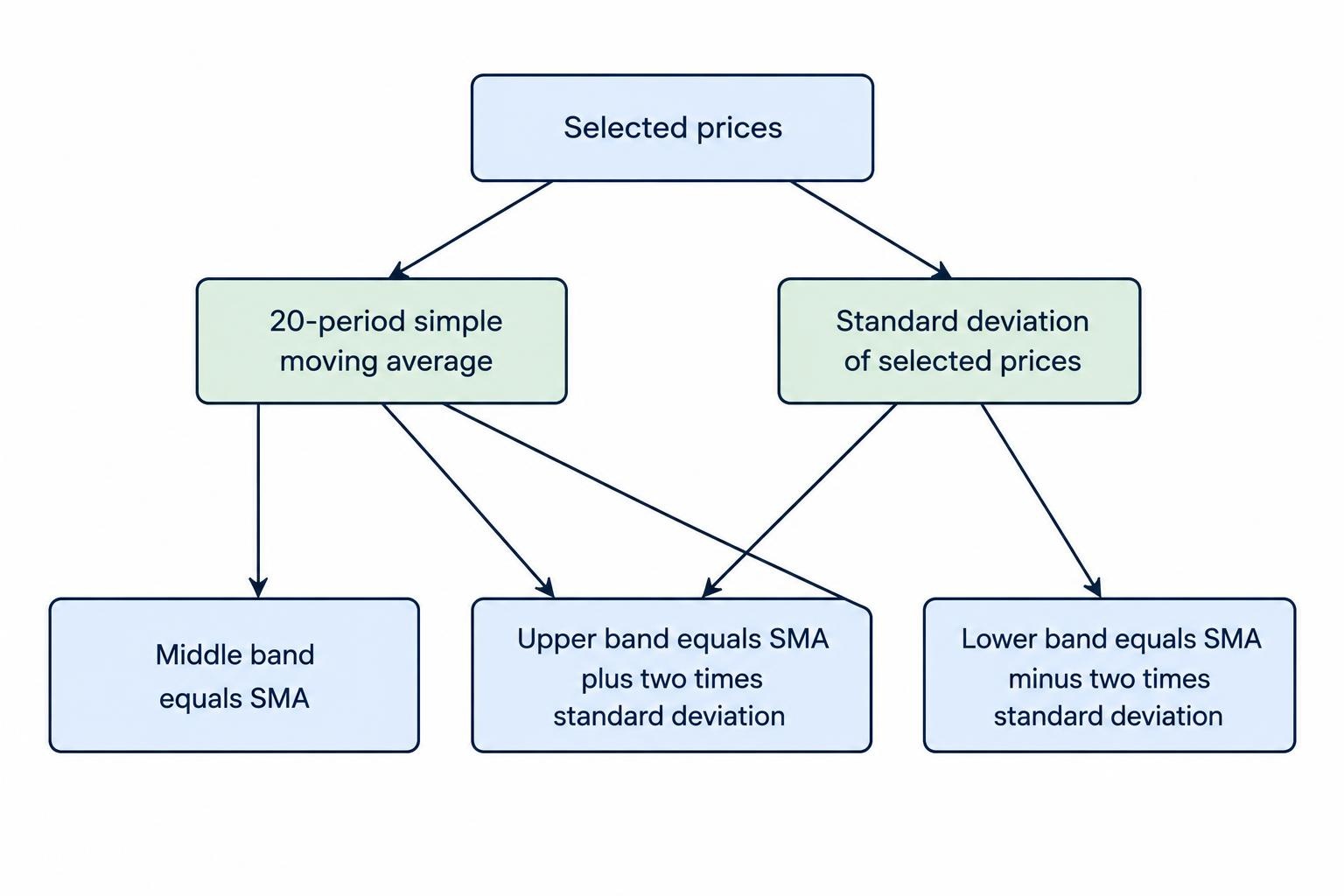
With population standard deviation, the calculation takes each price’s difference from the mean, squares those differences, averages them across all observations and takes the square root. A sample-standard-deviation implementation divides the sum of squared differences by one fewer observation, producing a somewhat different result. Confirm the convention and price source used by the software if exact signals need to match between platforms. As each new observation enters a rolling window, an older one leaves, so band width can change because old extremes disappear from the calculation. A narrowing channel does not necessarily mean that the current market has just become safer or that a directional move is about to begin immediately.
| Component | Standard setting or calculation | Practical interpretation |
|---|---|---|
| Middle band | 20-period simple moving average | Reference average for the selected window |
| Upper band | Middle band plus two standard deviations | Relatively high price boundary under that calculation |
| Lower band | Middle band minus two standard deviations | Relatively low price boundary under that calculation |
| BandWidth | Band separation divided by the middle band | Normalised measure of band width |
| %B | Price minus lower band, divided by band separation | Position of price relative to the bands |
Why two standard deviations do not provide a 95% forecast
The familiar statement that roughly 95% of observations fall within two standard deviations belongs to a normal-distribution model with appropriate assumptions. A rolling band around recent market prices is not automatically such a model, nor is it a prediction interval for the next price. Financial price behaviour, changing conditions and the dependence between observations prevent that shortcut from establishing a trading probability. John Bollinger’s own rules caution against making statistical assumptions from the indicator’s use of standard deviation. A move outside the bands therefore does not prove that a return inside is almost certain. It also does not justify enlarging a position on the assumption that an outside-band price must be an exceptional mistake.
There is another practical complication: the bands themselves move as new prices arrive. A trader might buy below the lower band and later see price back inside the channel without making a profit, because the lower band and middle average have moved down. Likewise, a short position can remain unprofitable even after a previously stretched price returns inside a rising channel. Test outcomes using actual entry and executable exit prices, rather than recording whether the market eventually touched a band or returned to the average. A successful description of indicator behaviour is not the same as a successful trade, particularly after the spread, financing and any slippage have been accounted for.
Understanding BandWidth and %B
BandWidth makes the distance between the bands easier to compare over time. A common percentage calculation is (upper band − lower band) ÷ middle band × 100, as shown in the StockCharts BandWidth documentation. With bands at 104 and 96 and a middle line at 100, BandWidth is 8%. Some displays use the decimal equivalent, 0.08, so check the scale before writing a threshold rule. “Narrow” should normally be assessed against the same market’s own history and timeframe. A value that is unusually low for one instrument can be routine for another. This normalisation also becomes unsuitable or unstable when the middle value is zero or very close to it.
The %B calculation is (price − lower band) ÷ (upper band − lower band). It equals zero at the lower band, 0.5 at the middle and one at the upper band; prices outside the channel can produce values below zero or above one. The StockCharts %B documentation explains this measure. With a price of 103 and bands at 96 and 104, %B is 7 ÷ 8, or 0.875. This describes location, not an 87.5% probability of any outcome. Some platforms multiply the result by 100. Where both bands coincide, the denominator is zero, so the implementation needs a convention rather than treating the calculation as an ordinary valid reading.
Band touches, closes outside and walking the bands
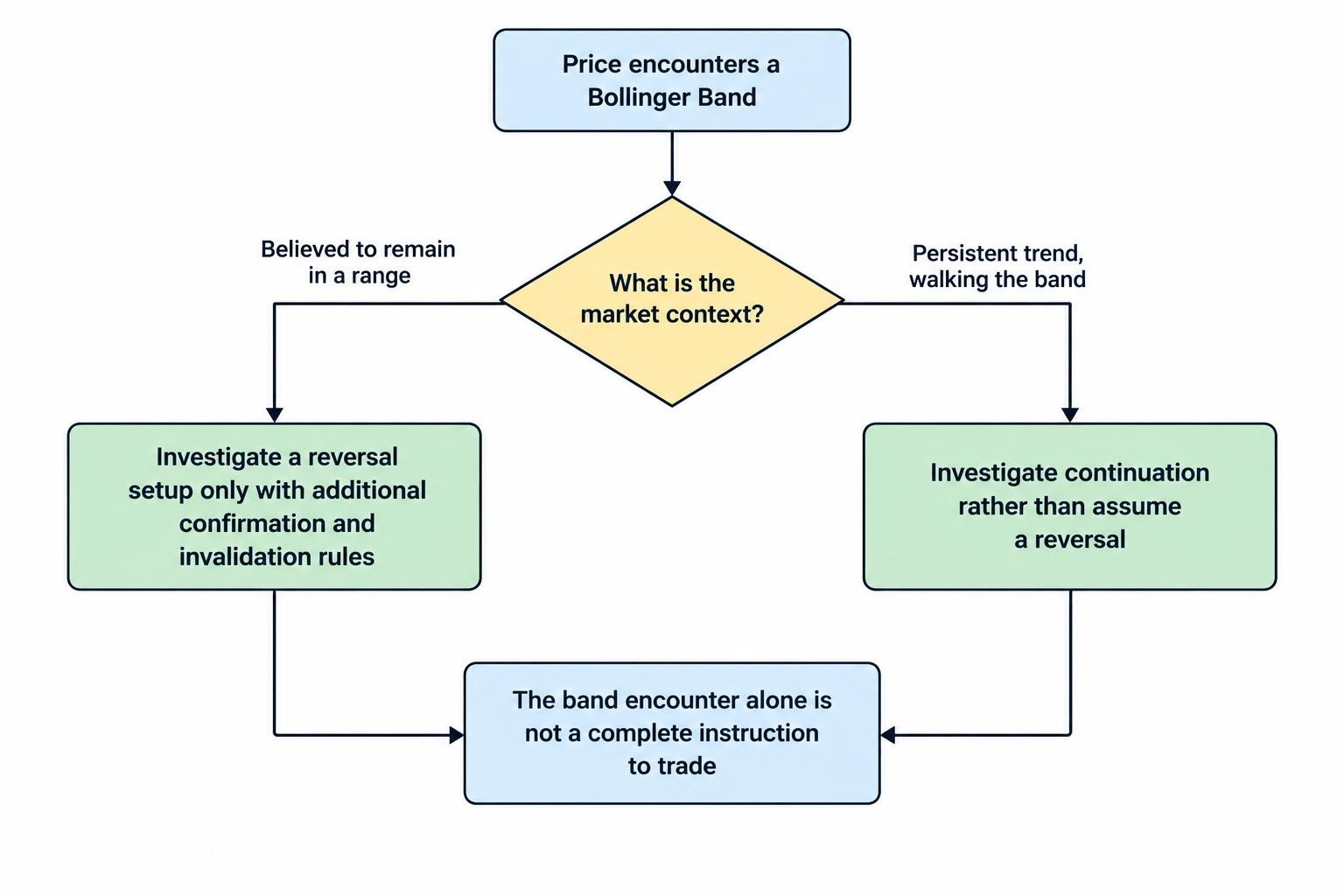
An intrabar touch, a completed close outside a band and a later close back inside are different events. A candle can briefly cross the upper boundary and finish well below it, while the band itself also changes during the candle. Rules must specify which event matters and whether the comparison uses the current completed band or the previous bar’s band. John Bollinger’s published guidance explicitly distinguishes band touches from trading signals. Buying every lower-band contact or selling every upper-band contact skips the question of why that contact occurred. The same observation can accompany an ordinary range fluctuation, a new trend or a sudden repricing after an announcement.
During a strong upward trend, price can repeatedly trade near the upper band; the equivalent can happen along the lower band in a decline. This is often called walking the bands. Selling each upper-band encounter can then create a series of losses while the market continues rising. A trend trader may instead interpret persistent upper-band activity as a reason to examine continuation setups, subject to price structure and an acceptable entry. That interpretation is still a hypothesis rather than a promise. Decide before entering whether the method seeks a reversal or continuation. Reclassifying an unsuccessful reversal trade as a long-term trend position changes the intended exposure without testing or planning the new trade.
Bollinger Bands settings and timeframes
The conventional 20-period, two-standard-deviation settings provide a starting point, not a universal optimum. Twenty periods means twenty bars on the chosen chart: twenty five-minute observations differ from twenty daily observations. Changing the period alters both the moving average and the dispersion being measured. Changing the multiplier alters how far the outer bands sit from the average. A wider multiplier generally reduces band contacts but does not prove that the remaining contacts have greater predictive value. Assess changes through complete entry and exit rules. Selecting a setting because it neatly captures a few past turning points can create an attractive chart while providing little evidence about the next series of trades.
Keep the instrument, session and source data consistent. Bands calculated from a cash index need not match those calculated from its futures contract or a provider’s spread betting price. Daily candles can also differ when session cutoffs differ. Record whether the chart shows bid, ask, midpoint or underlying-market prices, and whether the indicator uses closes or another input. A long spread bet closes at the executable sell price, while a short closes at the executable buy price; a chart touch does not necessarily establish that the relevant exit was available. If using a higher timeframe as a filter, distinguish its latest completed candle from the changing values of the current unfinished candle.
Bollinger Bands spread betting strategies
Range trading and mean reversion
A range method might investigate a long position when price tests established support near the lower band and subsequently closes back inside. The middle band or a predetermined price level could then provide an exit reference. The short version would investigate resistance near the upper band. Those observations need a separate reason to believe the market is still ranging, along with a price level showing that the assumption has failed. The band alone does not establish either condition. Our guides to range trading and mean reversion explain the broader reasoning. The main danger is continuing to expect another rebound after price has started a sustained move beyond the previous range.
Squeeze and breakout trading
A squeeze describes bands that have become relatively narrow, often measured using BandWidth compared with its earlier values. It can identify a market to watch for a change in activity, but it does not specify when expansion will arrive or whether price will rise or fall. A testable breakout method might require BandWidth to have been in a low historical percentile, then wait for a completed price break beyond a defined range. The percentile, comparison window and entry rule must be chosen before examining outcomes. The breakout trading guide covers execution after a break. A narrow channel can persist, and the first apparent escape can reverse instead of developing into a durable move.
Trend continuation and pullbacks
A continuation approach can combine a rising middle band, higher price highs and lows, and pullbacks that do not break the previously defined trend structure. The bands then describe where price sits within that advance, rather than instructing the trader to oppose every extreme. A possible entry might follow a pullback and renewed upward price movement, with the stop placed where that setup fails. In a falling market, the logic is reversed. The trend trading guide explains the wider approach. A pullback to the middle band is not automatically support: it is a meeting with an average that can itself turn lower. The executable entry and downside exposure still need to be assessed independently.
| Approach | Illustrative role for the bands | Additional requirement | Common failure |
|---|---|---|---|
| Range trading | Locate a relative extreme near a range boundary | Evidence that the range remains intact | Price breaks out and keeps moving against the reversal trade |
| Squeeze breakout | Identify contraction before an entry trigger | A defined directional price break and execution rule | The initial break reverses or offers a poor entry price |
| Trend continuation | Describe pullbacks and persistent directional behaviour | A price trend and a clear invalidation level | An ordinary-looking pullback becomes a reversal |
| Exit management | Provide an average or band-based exit reference | Rules for updating the reference and controlling losses | The moving reference changes the expected outcome |
W-bottoms, M-tops and relative price extremes
Bands can also help describe two-stage turning patterns. In a hypothetical W-bottom, the first low occurs outside the lower band, price rebounds, and a second low occurs inside the then-current lower band even if its absolute price is slightly lower. A later break above the intervening rebound high could be chosen as a separate trigger. An M-top reverses that general structure around the upper band. These are pattern definitions to investigate, not evidence that a reversal must follow. The second low or high often needs later candles for confirmation, so a historical test must preserve that delay. A pattern recognised only after a strong recovery cannot justify pretending that entry occurred at its lowest point.
Practical example: buying an index near the lower band
Assume a hypothetical index has an established range, with support around 9,770–9,780 and resistance above 9,900. On the selected chart, price tests support near the lower band and then a completed candle closes back inside the channel. The available quote is 9,800 to sell and 9,802 to buy. A trader buys at 9,802 for £0.50 per point, places an ordinary stop at 9,752 and sets a fixed target sell price of 9,902. The stop is 50 points below entry, giving £25 of planned price risk. The target is 100 points above entry, giving £50 of potential price profit before any separate charges. Nothing in the band contact establishes the probability of either outcome.
The target is fixed in price in this example; it is not automatically moved whenever the middle or upper band changes. Immediately closing at the unchanged sell quote of 9,800 would lose £1, because the opening spread is already reflected in the dealing prices. Assume £2 of funding over the eventual holding period and no other separate charges. Closing at the 9,902 target produces £48 net profit, while an earlier exit at 9,812 produces only £3 after funding. Closing at the original entry price produces a £2 loss. Cash break-even requires an executable sell price of 9,806. Actual funding varies with the contract, direction, rate and time for which the position remains open.
| Outcome | Executable sell exit | Price profit or loss | Assumed funding | Net result |
|---|---|---|---|---|
| Fixed target reached | 9,902 | £50 | £2 | £48 |
| Early exit with a small gain | 9,812 | £5 | £2 | £3 |
| Exit at the entry price | 9,802 | £0 | £2 | −£2 |
| Ordinary stop fills as planned | 9,752 | −£25 | £2 | −£27 |
| Gap through the stop | 9,702 | −£50 | £2 | −£52 |
If the market gaps through the ordinary stop, execution can occur below the requested level. In the final row, the price loss doubles from the planned £25 to £50, before funding. A lower band that expands or moves down during the decline does not reduce that cash loss. Nor should the trader widen the stop merely because the updated indicator makes the position appear less stretched. A guaranteed stop, where available and subject to its terms, can address execution beyond the agreed stop price, but charges and restrictions need to be included. Read the guides to stop losses, guaranteed stops and gap risk alongside any band-based entry method.
Practical example: selling a forex breakout after a squeeze
Suppose EUR/USD has formed a defined narrow price range while BandWidth is low relative to its recent history. A completed hourly candle then closes below both range support and its lower Bollinger Band. An illustrative method permits a short after that event, provided the available price remains within the planned entry range. The quote is 1.0840 to sell and 1.0842 to buy. The trader sells at 1.0840 for £0.50 per pip, with one pip defined here as 0.0001. A buy-side stop at 1.0890 is 50 pips away, giving £25 of planned price risk. A target buy price of 1.0740 offers a possible 100-pip gain, worth £50 before separate charges.
If the target is reached and funding costs £3, the net profit is £47. A smaller exit at a buy price of 1.0830 gives £5 of price profit and £2 after funding. If the apparent breakout fails and the stop fills at 1.0890, the net loss is £28 including the assumed charge. A gap to an executable buy price of 1.0940 produces a £53 net loss. The direction was supplied by the entry rule, not predicted by the earlier squeeze. Check whether the contract’s point corresponds to a pip or a smaller increment, and verify financing terms: a short spread bet does not automatically receive a funding credit. Different holding periods would also change the assumed costs.
Stops and position sizing: the band is not a loss budget
Start with the planned executable entry and the price level that invalidates the trade. In the index example, a £25 price-risk budget divided by the 50-point stop distance gives £0.50 per point. If the same budget must cover the assumed £2 funding charge, only £23 remains for the planned price loss, giving £0.46 per point before allowing for other costs or slippage. A minimum permitted stake may make that trade unsuitable for the budget. The position sizing guide explains the calculation. A narrow band can produce a close technical reference, but it does not guarantee that future price movement or a news-driven gap will remain small enough to fit it.
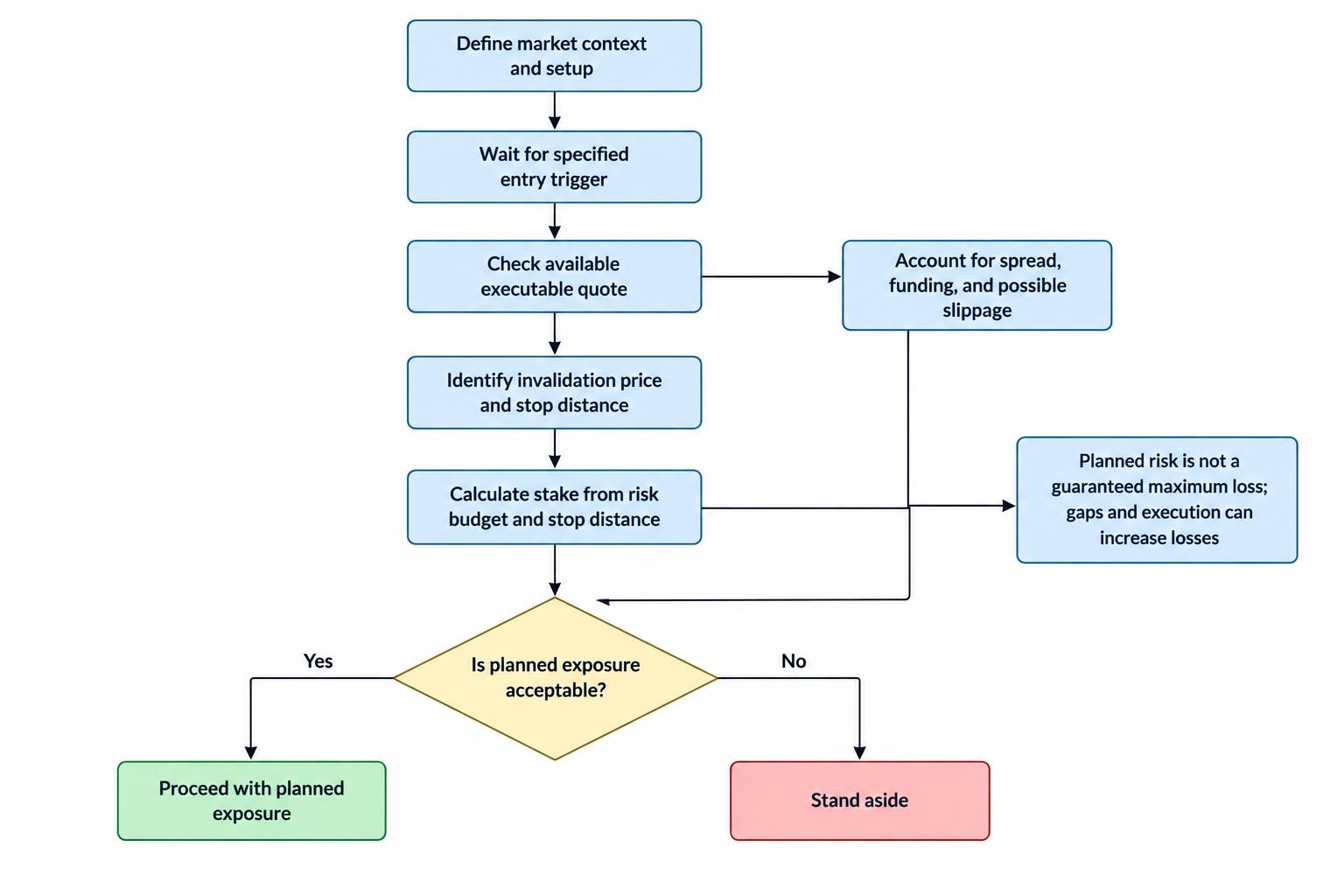
Using an outer band as a stop reference requires rules about updates. A lower band can move down while a long trade loses money, so automatically following it may increase the loss allowed after entry. A trailing-stop method should state whether a protective level may ever move away from the current price, and how the actual order is updated. Account for other positions as well: several band breakouts across related indices can reflect the same market event. The portfolio correlation guide addresses this concentration. Treating every signal as independent can underestimate the combined loss if the same unexpected development reverses several trades at once, even when each individual stake initially appears modest.
Margin and leverage with a Bollinger Bands trade
At 9,802 and £0.50 per point, the hypothetical index position represents approximately £4,901 of market exposure. An assumed 5% initial margin requirement would require £245.05. This is separate from the planned £25 price loss and does not cap the position’s possible loss. The FCA’s retail CFD rules specify a 5% minimum initial margin for major stock indices, with different minimums for other categories; firms can require more. Check the actual instrument and account terms rather than transferring that percentage to every market. Sufficient opening margin only establishes that the position can be opened under those terms, not that the stake, stop distance or combined account exposure is appropriate.
The same FCA rules require account-level closeout when net equity falls below 50% of required margin, as soon as market conditions allow. Negative balance protection for covered retail accounts limits liability to funds in the relevant account, but does not protect deposited trading money from being lost. Neither provision guarantees an individual stop price. An account closeout can also occur before the band-based exit originally planned by the trader. Monitor available funds, unrealised losses and the margin required across all positions, particularly through announcements or overnight holds. Chart conditions alone cannot reveal whether account-level constraints will force the trade to end before its intended technical exit occurs.
Costs and the problem of small expected moves
Range trades often seek relatively short moves, making the dealing spread large compared with the intended reward. Breakout trades can face wider spreads or slippage precisely when price accelerates. Positions held beyond a funding cutoff can also incur financing, and some short exposures involve borrowing costs. The FCA’s review of CFD providers’ price and value examines trading costs including overnight funding and their relationship to underlying exposure. Assess the product over the planned holding period instead of looking only at its headline spread. A visually clear move from a lower band to a middle band can leave little net profit if the entry arrives late or the cost of holding the position is high.
For a hypothetical strategy winning half its trades, suppose the average price profit is £30 and the average price loss is £20. The average result before separate charges is 0.50 × £30 minus 0.50 × £20, or £5 per trade. Average additional costs of £2 reduce that to £3. If a moving middle-band exit or delayed entry reduces the average winner to £22 while losses stay unchanged, the result becomes £11 minus £10 minus £2, or a £1 average loss. A high proportion of trades that eventually return inside the bands does not resolve this problem. Evaluate actual gains, losses, costs and drawdowns using the same entry and exit rules throughout the sample.
Which traders and markets do Bollinger Bands suit?
Bollinger Bands may suit traders who want to describe relative price position and changing dispersion within a written strategy. They can support intraday and multi-day methods, but the timeframe needs to match the trader’s availability. A five-minute reversal method can require frequent decisions, while a daily continuation method may involve financing and exposure to overnight gaps. The distinction between day trading and swing trading therefore extends beyond changing the chart interval. Alerts can draw attention to a condition, but they do not assess the quality of the quote or the suitability of the stake. A trader who cannot follow the required decision schedule needs a different process rather than an expectation that alerts will perform the analysis.
The indicator can be applied to shares, indices, currencies and commodities, but the same band settings do not make their risks interchangeable. An earnings announcement can reprice a share, an interest-rate decision can move a currency pair and a supply disruption can move a commodity. Bands respond when those developments enter the price data; they do not anticipate their content. Understand the underlying instrument, session and contract before relying on its chart. Bollinger Bands are less useful as a standalone solution for someone seeking exact tops, guaranteed reversals or a reason to avoid learning risk management. A convenient display does not make leveraged spread betting appropriate for a person unable to tolerate losing the funds deposited.
Advantages and disadvantages of Bollinger Bands
The main practical advantage is that the bands adapt their width to the selected price data instead of imposing a channel with a permanently fixed distance from an average. BandWidth and %B can make visual observations measurable, helping traders record and test consistent rules. The tool can also serve different purposes, including identifying contraction or describing a trend pullback. That flexibility creates a weakness when traders change interpretations after seeing the outcome. The same upper-band contact can be labelled bearish by a reversal trader and bullish by a trend trader. Without a prior rule, the indicator can explain almost anything afterwards. Its usefulness therefore depends on clearly choosing and testing the role it plays.
| Advantage | Limitation to assess |
|---|---|
| Width responds to recent price dispersion | Past dispersion does not cap future movement or gap size |
| Defines relative high and low positions | Does not measure fair value or guarantee a reversal |
| BandWidth makes contraction measurable | A squeeze does not determine direction or timing |
| %B provides a numerical location measure | It is not a probability or independent confirmation |
| Can support several trading approaches | Switching interpretations can make the strategy inconsistent |
Combining Bollinger Bands with other technical tools
Choose additional tools to answer clearly different questions. Support and resistance can identify previously important price areas, while RSI or MACD can add a stated momentum condition. These indicators still derive from price, so their agreement is not equivalent to independent evidence from several unrelated sources. BandWidth and %B are calculations from the same bands and must not be counted as separate confirmations either. If adding volume, check what it represents: underlying exchange volume and a provider’s tick count are different datasets. Compare the expanded method with its simpler version to establish whether the extra condition improves results enough to justify fewer trades or later entries.
Bollinger Bands also differ from ATR and from other price channels. ATR uses true ranges incorporating the current high and low and gaps relative to the previous close; conventional Bollinger Bands use dispersion of closing-price levels. A steady trend can spread those closes around their average even when individual candle ranges are fairly regular. Common Keltner Channel implementations use an average with ATR-based boundaries, while Donchian Channels use highs and lows over a chosen period. These constructions need not identify the same breakouts or stop distances. Indicator names should therefore be recorded precisely, especially when a template combines Bollinger Bands with another channel to define a particular type of squeeze.
How to get started with a Bollinger Bands method
Begin with one market, one timeframe and one purpose for the bands. An educational exercise could examine completed closes back inside the lower band near separately defined range support. Write down how the range is identified, which candle confirms entry, the acceptable dealing price, the stop, the target or exit rule and the stake calculation. Include conditions for standing aside, such as a scheduled announcement or a spread above the chosen limit. Before funding a live account, follow the FCA’s guidance on checking authorisation and relevant permissions. Those checks concern the provider and its permissions; they do not validate the strategy or protect a trading position from adverse market movements.
Review historical setups in sequence, including failed reversals, failed breakouts and periods when no trade qualified. Then practise the written rules in a demonstration environment, recording the quote available after the confirmed signal rather than assuming execution at the prior candle’s close. Demo practice can improve familiarity with order handling but does not fully reproduce live fills or the pressure of losing money. Keep a journal of the band values, price context, trigger, stake, stop, entry, exit and charges, together with any rule changes or deviations. This helps distinguish a method that performs poorly from an execution mistake. A collection of screenshots showing prices bouncing neatly from the bands cannot provide that distinction.
Testing the strategy without fitting it to the past
Changing periods, multipliers, squeeze thresholds, trend filters and exits creates many possible strategies, increasing the chance that one looks impressive by accident. The Probability of Backtest Overfitting examines this problem in investment strategy selection. Record the alternatives tried, evaluate on data not used to choose the rules and examine different market conditions. Repeatedly adjusting the strategy after consulting the evaluation data weakens that separation. Prefer an economically and operationally plausible method whose results are not dependent on one exact parameter combination. Even then, favourable historical results do not establish future profitability. The relevant question is whether the apparent advantage survives realistic assumptions and further observation, rather than whether enough adjustments can make a backtest attractive.
Pay particular attention to when band values were known. A close below the previous bar’s lower band and a close below the newly recalculated lower band are different tests. A completed-bar rule also cannot assume an earlier entry during that candle. If both a stop and target are touched within one bar, the high and low alone may not reveal which occurred first; use suitable intrabar information or a stated conservative assumption. Include bid–ask differences, funding, slippage and unavailable trading periods. Review net results, drawdowns and losing sequences as well as win rate. A method can look tolerable on average while exposing the account to an unacceptable occasional loss or a prolonged run of unsuccessful trades.
Frequently asked questions about Bollinger Bands spread betting
Does touching the lower band mean you should buy?
No. A lower-band touch means price has reached a relatively low level under the indicator’s current calculation. It can occur during a range fluctuation, a developing downtrend or a rapid adjustment to new information. A buy method needs additional definitions for the market context, entry event and price level that invalidates the expected rebound. Waiting for a close back inside is one possible condition, but that is a different rule from buying the initial touch and it still can fail. Evaluate each complete approach separately. Neither the band contact nor a later return inside establishes that the available dealing prices will produce a profit after costs and possible adverse execution.
What are the best Bollinger Bands settings for spread betting?
There are no universally best settings. Twenty periods and two standard deviations provide the conventional starting point, but their suitability depends on the instrument, timeframe, source data and the intended entry and exit rules. Wider bands reduce some contacts; shorter periods change the average and dispersion more rapidly. Neither adjustment establishes that the remaining trades are better. Compare complete strategies under consistent execution and cost assumptions, and avoid repeatedly tuning settings until past turning points look neatly captured. Record the standard-deviation convention and any changes to the moving-average type as well. Two templates showing the same period and multiplier may still differ if their underlying calculations or price inputs are different.
Can you use the middle band as a profit target?
The middle band can be an exit reference, but a strategy must state whether its value is fixed at entry or updated during the trade. In a declining market, the average can move down towards a long position’s entry or below it, reducing or eliminating the originally expected profit. A later touch of that moving average is therefore not proof of a successful mean-reversion trade. Calculate the actual executable exit price and deduct all costs. It may also be sensible within a tested method to define a time exit or other invalidation condition, rather than waiting indefinitely for a meeting with the average while funding and market exposure continue to accumulate.